Geomorphometry, unbound from planar grids.
GGEE performs third-order geomorphometric analysis directly on the WGS 1984 reference ellipsoid within Google Earth Engine—eliminating the need for map reprojection, bypassing the conventional 3×3 moving window ceiling, and requiring zero lines of code. Simply define a region of interest, set a scale-free moving window (from 5×5 up to 51×51 pixels and beyond), and export geodetically exact morphometric models at a scale of up to ten trillion pixels.
Global DEMs use spheroidal equal angular grids. Classic algorithms assume plane square grids.
Global DEMs—such as SRTM, ALOS, and Copernicus—are natively distributed on spheroidal equal angular grids. While their angular spacing remains constant, the physical size of each cell intrinsically shrinks with latitude. However, classical techniques (e.g., the Evans-Young method) and the standard GIS tools built upon them, assume a uniform plane square grid. Conventional workflows that ignore this geometric mismatch typically resort to one of two flawed workarounds.
Reprojection and Resampling
Reprojecting global data into a planar coordinate reference system (e.g., UTM) forces a raster-wide interpolation. As noted in geomorphometric theory, any interpolation inherently introduces new errors and artifacts. These artificial anomalies fundamentally corrupt the derivation of higher-order variables, particularly second-order curvatures and third-order deflections.
Ignoring the Grid Geometry
Because meridians converge toward the poles, a true ground cell forms a spheroidal trapezoid rather than a perfect square. Applying plane square-grid algorithms to these cells produces topographic shear error—a systemic distortion in slope gradients and flow directions that intensifies at higher latitudes.
Scaled Spheroidal Convolution
GGEE overcomes these limitations by fully decoupling the analytical geometry of the grid (pixel arrangement) from the differential geodesy of the ellipsoid (true physical dimensions). This decoupling is executed through a highly optimized three-step architecture.
Single Inversion, Universal Application
A third-order Taylor polynomial requires estimating 10 unknown differential parameters. GGEE solves the least-squares design matrix for the selected moving window size exactly once, over a dimensionless unit grid. The resulting pseudo-inverse is retained as a fixed bank of 10 spatial convolution kernels, entirely eliminating the computationally prohibitive need for per-pixel matrix inversions.
Dynamic Scaling via Morozov's Equations
The dimensionless kernels are convolved across the DEM to extract raw grid derivatives. GGEE then applies Morozov's equations for the WGS84 ellipsoid to calculate the meridional (M) and prime-vertical (N) radii of curvature dynamically for every pixel. Fast, parallel map-algebra division rescales the raw derivatives into true physical units—crucially, after the convolution phase, ensuring extreme computational efficiency.
The Y-Axis Mirror Rule
In standard raster data formats, row indices typically increase downward (southward), contradicting the Cartesian Y-axis which increases northward. To correct this, GGEE automatically inverts the sign of any derivative containing an odd power of the Y-variable. This ensures that orientation-dependent variables, such as slope aspect and flow routing, remain precisely aligned with true geographic north.
Beyond Conventional Terrain Analysis
While traditional desktop GIS and earlier cloud-based packages addressed aspects of geomorphometry, GGEE redefines the standard by simultaneously upgrading the moving window scale, polynomial order, and reference geodesy.
| Dimension | Desktop GIS ArcGIS · SAGA · GRASS |
Earlier cloud tools e.g. TAGEE on GEE |
GGEE |
|---|---|---|---|
| Moving Window | Fixed 3×3 | Fixed 3×3 | Scale-free, any odd size 5×5 → 51×51+ |
| Surface model | Bivariate 2nd-order polynomial | Bivariate 2nd-order polynomial | Bivariate 3rd-order Taylor polynomial, 10 parameters |
| Reference geometry | Requires reprojection to a planar CRS | Spherical approximation, Haversine distances | Ellipsoid-native (WGS84), dynamic Morozov M/N radii of curvature |
| Selectable outputs | Toolbox-dependent, mostly 1st/2nd order | Limited fixed set | 26 outputs: 22 morphometric layers + 4 classifications |
| Interface | Desktop menus / scripting | JavaScript API, code required | No-code browser app — draw, select, export |
26 Selectable Layers Across Four Categories
GGEE leverages Google Earth Engine's lazy evaluation: each output is a band within a unified image. The system computes only the specific variables you request, ensuring zero computational overhead for unselected layers.
First-Order Variables
Second-Order Variables (Curvature System)
Third-Order Variables (Deflections)
Nonlocal Variables & Landform Classifications
22 continuous morphometric variables + 4 classification layers = 26 selectable outputs
Four Classification Systems, Four Analytical Perspectives
GGEE utilizes the derived continuous morphometric variables to drive four independent landform classification typologies. Each system translates differential geometry into categorical geomorphological classes, tailored to specific research objectives.
Landscape Position
Applies standard-deviation thresholds to a scale-dependent Topographic Position Index (TPI) to categorize pixels into valleys, lower slopes, flat areas, middle slopes, upper slopes, and ridges.
Elementary Surface Forms
Utilizes the signs of mean curvature and Gaussian curvature to partition the terrain into fundamental geometric forms: peaks, ridges, saddles, planes, and basins—rooted purely in differential geometry.
Flow Behavior
Based on the signs of horizontal and vertical curvatures, this 9-class system captures the kinematics of gravity-driven flows, identifying areas of flow acceleration, deceleration, convergence, or divergence.
Comprehensive Typology
Integrates the signs of Gaussian, mean, and difference curvatures to provide the most complete, fine-grained landform typology in the suite.
Planetary Scale, Rigorously Validated
Larger moving windows and higher-order mathematics inherently introduce specific failure modes. Rather than leaving these complexities to the user, GGEE integrates robust, automated safeguards to ensure mathematical and geometric integrity at planetary scales.
Float64 Precision Throughout
While Earth Engine often defaults to lower precision to save memory, GGEE forces Float64 (double precision) across the entire computational pipeline. This ensures that delicate classification zero-crossings (e.g., H ≈ 0, K ≈ 0) do not dissolve into computational noise.
Epsilon Flat-Threshold Masking
A user-tunable epsilon value isolates genuine flat areas from residual sensor noise. This crucial masking occurs before any ratio divides by a near-zero slope, effectively preventing spurious, infinite curvature spikes.
Dynamic Accuracy Guard
GGEE employs a closed-form Dirichlet-kernel identity to analytically suppress the majority of topographic shear error within each moving window.
If the residual shear exceeds 0.5%, GGEE issues a warning, suggesting a smaller moving window or a tiled Region of Interest (ROI).
10-Trillion-Pixel Ceiling
Exports are executed with maxPixels configured up to 1e13. Crucially, the original DEM transform is injected directly into the export engine, guaranteeing that the output morphometric grids remain perfectly aligned (pixel-shift free) with the source data.
Zero-Code Processing in Four Simple Steps
Define the Region of Interest (ROI)
Sketch a polygon or rectangle directly on the interactive map to precisely delineate your study area.
Configure the Moving Window
Specify any odd-integer dimension (≥ 5×5) for the scale-free moving window. The default is 11, offering an optimal balance between regional smoothing and local topographic detail.
Compute & Preview
Select any morphometric variable or landform classification from the 26-item suite. Inspect the real-time computation on the map before initiating large-scale exports.
Export to Google Drive
Export your results as a geodetically aligned GeoTIFF. The output strictly matches the source DEM's original transform, ensuring seamless integration into your downstream GIS workflows.
Rigorous Mathematical and Algorithmic Framework
GGEE is accompanied by a comprehensive technical document detailing its theoretical foundation. This includes the mathematical formulation of the third-order Taylor polynomial surface fit, WGS84 geodetic scaling via Morozov's equations, the derivation of the Dynamic Accuracy Guard, and an exhaustive interpretation reference for all morphometric variables and landform classifications.
- Mathematical Foundations: Bivariate third-order Taylor polynomial fitting, decoupling of grid geometry from differential geodesy, and analytical topographic shear-error correction.
- Operational Workflow: Region of Interest (ROI) delineation, scale-free moving window strategies, and geodetically aligned raster exports.
- Geomorphological Interpretation: Detailed reference guides for all 22 continuous morphometric variables and 4 categorical landform classification systems.
The GGEE Interface within Google Earth Engine
Experience GGEE exactly as it operates within your browser—requiring no local desktop installation and no exposed script editors. The streamlined left panel houses the complete analytical interface, while the right panel provides a real-time, interactive map preview.
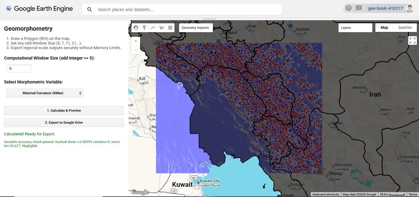
The status indicator beneath the control panel displays the Dynamic Accuracy Guard reporting in real time. For this specific execution, at the Region of Interest's (ROI) highest latitude, the residual topographic shear remaining after the Dirichlet-kernel correction was mathematically negligible—well below the 0.5% warning threshold.
Geomorphometry (Companion Text)
A peer-reviewed academic text detailing the theoretical foundations, local and nonlocal morphometric variables, and practical applications that power both the GGEE platform and the Geomorphometry Toolbox.

Geomorphometry (ژئومورفومتری)
Authored by Javad Khanifar, this academic work provides an in-depth exploration of continuous surface modeling, flow-routing algorithms, and automated landform classification systems — the same foundations that GGEE's engine implements at planetary scale.
Contact the author for academic inquiriesJavad Khanifar

An academic lecturer, researcher, and interdisciplinary specialist, Javad Khanifar’s expertise spans soil science and engineering, geomorphometry, remote sensing, and artificial intelligence. His research is dedicated to integrating cutting-edge computational methods into the geosciences and agricultural engineering. Both GGEE and its predecessor, the Geomorphometry Toolbox for ArcGIS Pro, are direct products of this ongoing applied research.
Common questions about GGEE
What is GGEE?
GGEE is a zero-code Google Earth Engine application designed to calculate morphometric variables—including slope gradient, the complete curvature system, deflections, Topographic Position Index (TPI), and landform classifications—directly on the WGS84 ellipsoid utilizing a third-order, scale-free surface model.
How does GGEE differ from conventional desktop GIS tools or previous cloud packages?
Conventional desktop GIS toolboxes and earlier cloud tools typically rely on a fixed 3×3 moving window and a bivariate second-order polynomial applied to a reprojected or spherical approximation. GGEE, conversely, utilizes a scale-free moving window (from 5×5 up to 51×51+), a 10-parameter third-order Taylor polynomial, and native WGS84 ellipsoid geodesy—all seamlessly accessible via a zero-code browser interface.
How many outputs does GGEE produce?
GGEE offers 26 strictly selectable outputs. This suite encompasses 22 continuous morphometric variables (comprising first-order variables, second-order curvatures, third-order deflections, and the nonlocal TPI), alongside 4 rigorous landform classification systems (Weiss, Gaussian, Efremov-Krcho, and Shary).
How can I access GGEE?
Access to the GGEE computational engine is currently contingent upon the establishment of joint scientific research initiatives, academic partnerships, or applied engineering projects. Please contact the principal developer, Javad Khanifar, directly to discuss collaboration and platform access.
Which DEMs are compatible with GGEE?
Standard global digital elevation models natively distributed on a spheroidal equal angular grid—such as SRTM, ALOS World 3D, and Copernicus GLO-30—are fully compatible with GGEE's architecture.
Inquiries Regarding GGEE or Joint Research Initiatives?
Reach out directly via email to discuss academic collaborations, technical inquiries, or to request access to the computational engine.